
The launch of the Coastal Zone Color Scanner (CZCS) aboard the Nimbus-7 spacecraft in the fall of 1978 ushered in the age of satellite ocean color measurement. During those early days one probably needed to be on the Nimbus Experiment Team with a requested target in mind in order to obtain a particular ocean color scene.

Figure 1: CZCS laserfax sheet

Figure 2: CZCS processing request
As the mission progressed a paper archive of low quality, black and white CZCS scenes began to accumulate. These laserfaxes (Figure 1), as they were known, were kept in a filing cabinet in the basement of a building at NASA's Goddard Space Flight Center. The Nimbus-7 mission operations folks would annotate these laserfaxes in the margin to indicate which portions of the data should be queued for further processing, but, due in part to the low quality of the images, significant numbers of cloud free areas of interest were often overlooked. If a researcher wanted to work with CZCS data for a region that was not initially selected for processing, they would have to make their way down to the basement of Building 3/14 at NASA/Goddard, find the appropriate file cabinet that contained the near real-times for the period of time that they were interested in and if they were lucky, had great eyesight and lots of stamina, they could go back through the laserfax files and highlight additional 2 minute blocks of scan lines to be processed (Figure 1 and 2).

Figure 3: CZCS level-1 transparency
Scenes that received further processing were stored on magnetic tape and photographically recorded and archived in transparency form (Figure 3). If a researcher wished to search the archive, they could come to Goddard and spend an afternoon or longer at a light table flipping through stacks of these transparencies in hopes of finding a scene that:
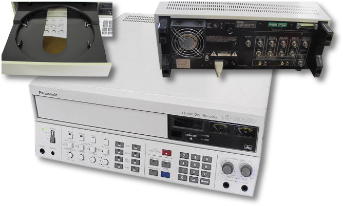
Figure 4: Three views of a Panasonic TQ-2026F optical disc recorder
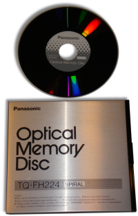
Figure 5: Panasonic optical memory disc and carrying case
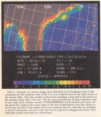
Figure 6: Sample CZCS browse image
By 1989, the entire digital archive of CZCS scenes (some 66,000 or so) had been migrated from 9-track tape to more recent, random access storage technology, and the majority of the scenes had been processed to derive sea surface chlorophyll fields that could be represented as pseudo-color images. We used a Panasonic TQ-2026F to record all of those images onto three Panasonic TQ-FH224 optical memory discs as individual NTSC frames. The Panasonic players could be commanded by computer via an RS-232 cable to seek to a specific frame, so we kept a record of that frame number along with the date and time that the scene was collected and the two latitudes and two longitudes that hemmed it in. Now, ocean color users in possesion of a computer, a Panasonic player, two monitors, and copies of the three CZCS browse discs could run a program that we wrote, enter four bounding coordinates and a date range, and be presented with a sequence of images whose bounding boxes overlapped their own search area. They could very rapidly step through the matching image frames displayed on their TV screens with single key strokes at their computer to indicate which scenes were clear or otherwise interesting enough to merit addition to their order list. Completion of a browse session resulted in a list of scene identifiers that could be sent to the archive at NASA for filling.
During the mid 1990's we began to develop ideas for a new type of ocean color browse tool. Two developments, in particular, led us to change the way that we implemented geographical searches and the way we presented search results to interested users.
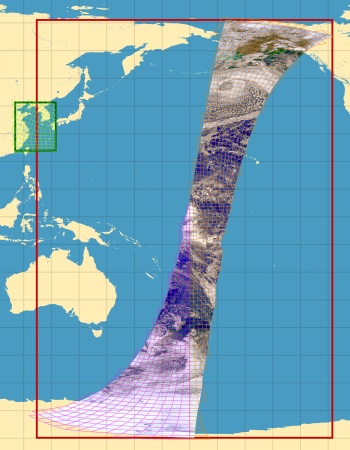
Figure 7:
A typical SeaWiFS GAC swath is enclosed in a red rectangle defined by the
scene's northern and southernmost latitudes and western and easternmost
longitudes. A search for data in the East China Sea (green rectangle)
would return this scene as a match using those metadata even though the
data do not come within 5000 kilometers of the green rectangle.
If the search were based on shared quadsphere bins (light green,
magenta, and orange outlines), there would be no match.
Note that the SeaWiFS swath is divided into two groups of quadsphere bins (magenta and orange) along the 180-degree meridian. This reflects the fact that the swath contributes to two different geographically determined data days.
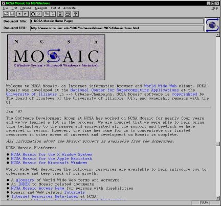
Figure 8: Screen shot of NCSA Mosaic
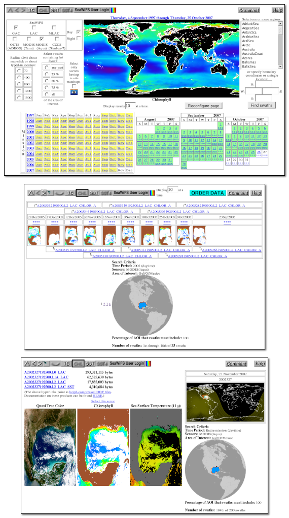
Figure 9:
Screen shots from
https://oceancolor.gsfc.nasa.govNo Remote Path MatchNo Remote Path Match/cgi/browse.pl
The interface pictured at right allows the user to select one or more time periods of interest by clicking on hyperlinks in a calendar or by selecting date ranges from pull-down menus. Geographical regions of interest can be selected from a list, via a click on a map, or by typing in sets of bounding coordinates. Programs running on our webserver encode the user's regions of interest as a list of quadsphere bin numbers (see below) which is then passed via a temporary database table and an SQL query to our MySQL database engine along with the user's specified time ranges. Thumbnail images of the scenes selected by the query get displayed on the user's computer along with hyperlinks to the full data files should the user wish to download any of them directly.
One day, a few years before SeaWiFS launched, I was contemplating ways of getting from a point on a map to a list of satellite scenes that included that point when I overheard Fred Patt discussing an equal area binning scheme called the quadrilateralized spherical projection or quadsphere. Fred came to our group from the Cosmic Background Explorer Project where that projection was used while looking away from Earth. His description of the quadsphere follows.
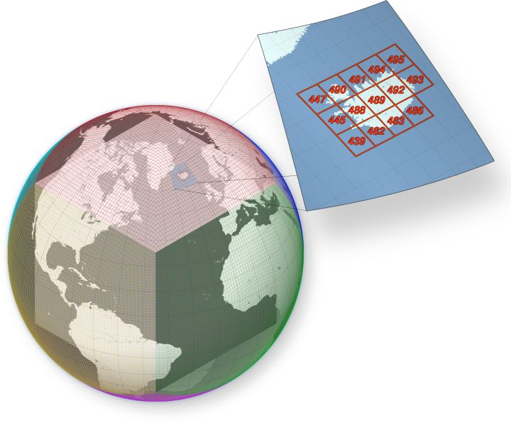 Figure 10:
This diagram shows quadsphere level-6 bin boundaries drawn on a
semi-transparent globe with the inscribed cube visible inside.
The outlines for quadsphere bin faces 0 through 5 are colored red,
green, blue, cyan, yellow, and magenta, respectively. The expanded
section shows the numbering of the bins that overlay Iceland.
Figure 10:
This diagram shows quadsphere level-6 bin boundaries drawn on a
semi-transparent globe with the inscribed cube visible inside.
The outlines for quadsphere bin faces 0 through 5 are colored red,
green, blue, cyan, yellow, and magenta, respectively. The expanded
section shows the numbering of the bins that overlay Iceland.
The Earth's surface is projected onto the faces of an inscribed cube using a curvilinear projection which preserves area. The sphere is divided into six equal areas which correspond to the faces of the cube. The vertices of the cube correspond to the cartesian coordinates defined by |x|=|y|=|z| on the unit sphere. The cube is oriented with one face normal to the North Pole and one face centered on the Greenwich meridian.
The faces of the cube are divided into square bins, where the number of bins along each edge is a power of 2, selected to produce the desired bin size. Thus the number of bins on each face is 2**(2*N), where N is the binning level, and the total number of bins is 6*2**(2*N). For example, a level of 10 gives 1024x1024 bins on each face and 6291456 (6*2**20) total bins, and on the Earth's surface the bins are 81 km**2 in size.
The bins are numbered serially, and the bin numbers are determined as follows. The total number of bits required for the bin numbers at level N is 2*N+3, where the 3 MSBs are used for the face numbers and the remaining bits are used to number the bins within each face. The faces are numbered 0-5 with 0 being the North face, 1 through 4 being equatorial with 1 corresponding to Greenwich, and 5 being South. Thus at level 10, face 0 has bin numbers 0-1048575, face 1 has numbers 1048576-2097151, etc.
Within each face the bins are numbered serially from one corner (the convention is to start at the "lower left") to the opposite corner, with the ordering such that each pair of bits corresponds to a level of bin resolution. This ordering in effect is a two-dimensional binary tree, which is referred to as the quad-tree. The conversion between bin numbers and coordinates is straightforward. The maximum practical bin level is 14, which uses 31 bits in a 32-bit integer and results in a bin size of 0.32 km**2.
The quad sphere limits the allowable bin sizes by requiring the bin dimenension of the cube face to be a power of 2, due to the binary indexing scheme. The advantage is that the bin numbering allows the resolution to be changed (by factors of two) simply by adding or deleting LSBs. This is particularly useful if it is desired to increase the bin size, for example to compare maps with different resolutions. This is performed simply by dividing the bin numbers by four for each factor of two increase in bin size.
The quad sphere faces can be displayed individually without remapping, with moderate distortion in the corners of the faces.
The quad sphere has an advantage in that the binary numbering scheme allows contiguous subsets of bins (either whole faces or quadrants of faces) to be accessed by simply specifying a range of bin numbers.
This, I thought, could be an elegant way of parcelling up the Earth's surface into small, numbered areas that I could then associate with satellite scenes and regions of interest.
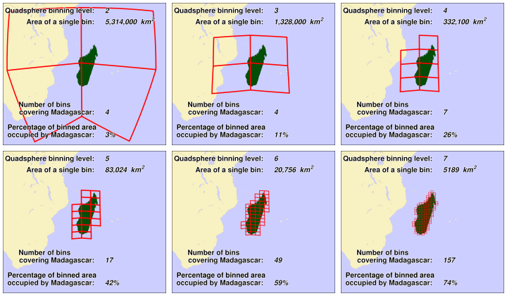 Figure 11:
As the quadsphere bin level increases, the area of individual
bins decreases, and the number of bins covering the same area
increases. Representation of the desired region of interest
(the island of Madagascar in this example) also becomes more
accurate as the bin level increases.
Figure 11:
As the quadsphere bin level increases, the area of individual
bins decreases, and the number of bins covering the same area
increases. Representation of the desired region of interest
(the island of Madagascar in this example) also becomes more
accurate as the bin level increases.
The typical MODIS scene overlays about 260 level-6 quadsphere bins; a typical SeaWiFS GAC swath overlays an average of around 1400 bins. The program that determines which bin numbers to associate with each scene gets all of its information from small browse files that are generated by the OBPG data system. In fact, all of the metadata used by the browse interface that I am describing come from these browse files which contain enough information to determine the location of each pixel in the subsampled browse scene.
The steps to determine which quadsphere bins overlay a given scene are as follows.
So, satellite data comes into our archive and gets processed. For each scene, at least one browse file is generated from which metadata are extracted. These metadata are inserted into tables in an ever-growing relational database (currently, a MySQL implementation). Between this database and the user sits the ocean color browse interface pictured above (Figure 9). When a user executes a search by clicking on the map or the Find swaths button, the browser code queries the database using the user's search parameters and returns the requested satellite scenes.
We have restructured our database tables a bit since I wrote what follows
and since I created the figure below. The
quadsphere table has gained a sen_id
(sensor identifier) field which points to a record in a new
sensors table that contains more information
about the missions that we support. The start_time,
station, width, height, sensor, and hide fields have moved out of the
granules table into a
scene_info table and have been linked with
additional foreign keys. The basic idea of the search is still the same,
however.
Norman Kuring
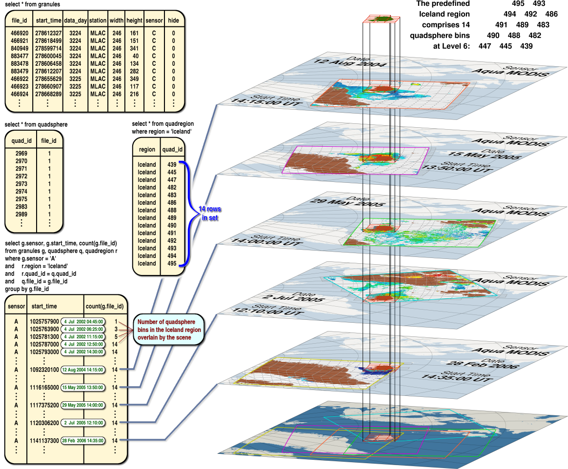
The diagram below illustrates a sample query in which a user is looking for Aqua-MODIS scenes that overlay the predefined Iceland region.
The first database table shown in the upper left is called
granules, and it contains the
following basic scene information.
file_idgranules
table to rows in other tables
start_timedata_daydata_day field will occasionally differ by one day from the date
encoded in the start_time field; note also that scenes
which span the geographical data day boundary will have two rows
in the granules table with the same
start_time but data days that differ by one.
stationwidth and heightsensorhide
The quadsphere table contains the
geographical coverage of each granule by associating each
file_id in the granules
table with a set of level-6 quadsphere bin numbers (quad_id)
each of which refers to a unique georaphical area.
The quadregion table stores, again
via level-6 quadsphere bin numbers (quad_id), the
geographical coverage of predefined regions such as Iceland.
The Iceland region comprises 14 bins and is shown in the figure
below and in Figure 10.
The query and results shown in the lower left portion of the
diagram below show how the aforementioned three tables can be
joined to return a set of rows that contain the information
needed to identify each paticular scene. (The scene start
times are translated in green to a more human-readable form.)
By using the group by clause in the query, the
browse code can help the user to further restrict her search,
say, to include only scenes that overlay all of the Iceland
region. Such scenes would have a value of 14 in the
count(g.file_id) column. Scenes that contained
at least 50% of the Iceland region would have values of 7
or greater in this column. Five of the scenes
selected by the query that do overlay all 14 Iceland quadsphere
bins have been mapped and displayed along the right side of
the diagram showing their relationship to the Iceland region.
All geographic searches are implemented in this way via
quadsphere bin numbers whether the lists of bins come from
predefined regions or from user clicks on the world map
(Figure 9) or from latitudes and longitudes typed in by
the user. Temporal searches make use of the data_day
field in the granules table
to exclude scenes that are outside the user's specified
date ranges.